Live drive, seed 1, real time. A car turns left across the junction. Our car stops and waits until 2 s after the other car leaves the camera's view. Inset: the bird's-eye grid that the planner reads.
The question
In the first part of the course our group wrote Trajecta, a Python library for lane detection, object detection and tracking, segmentation, sign recognition and vehicle control. In Webots it could follow one road. At a junction it lost the lane, and it could not read a traffic light or tell where it was on the map. On the city loop it completed 30% of the route.
In the second part we asked if the same library, extended and not rewritten, could drive the whole loop. One rule set the scope: the car uses only a camera, a range finder, GPS, an IMU, a gyro, wheel speed and a static map. The simulator’s ground truth goes only to the code that scores the drive. Localisation is then a real estimation problem, and no reported number depends on the car’s own estimates.
The system
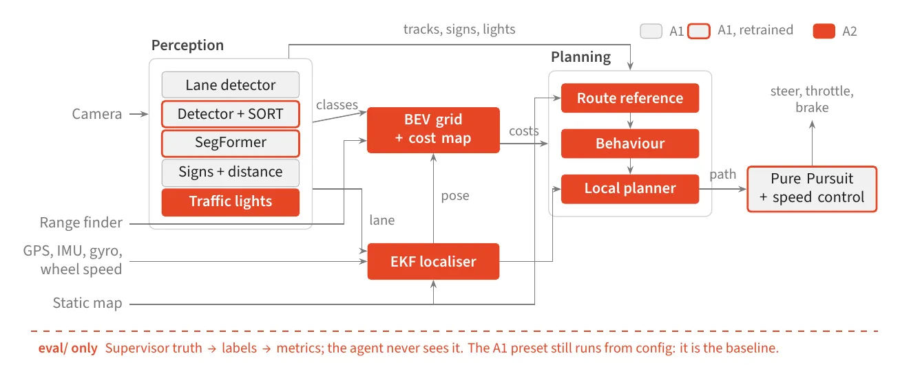
Grey: modules from the first part, used unchanged. Red outline: modules retrained on this world. Red: new modules. Ground truth stays below the dashed line.
Each stage is selected in a YAML preset. The original lane-following system is still a preset and serves as the baseline, so each comparison runs the same code with a different configuration. Simulator code stays in the adapter and the evaluation package, so the 1327 tests run without Webots, a GPU or model weights.
- My partThe shared types and protocols, the sensor adapter, the bird’s-eye-view grid and its cost map, the fine-tuned segmentation model, the live dashboard, and the integration and test runs of the whole system.
- TeammatesAmy Nguyen: localisation and grid tracking. Marium Haider: traffic lights, vehicle detection and distance. Ananth Rahul Somayaji: planning, behaviour and control. Wenqian Gong: the map and the evaluation harness.
From the camera to a grid
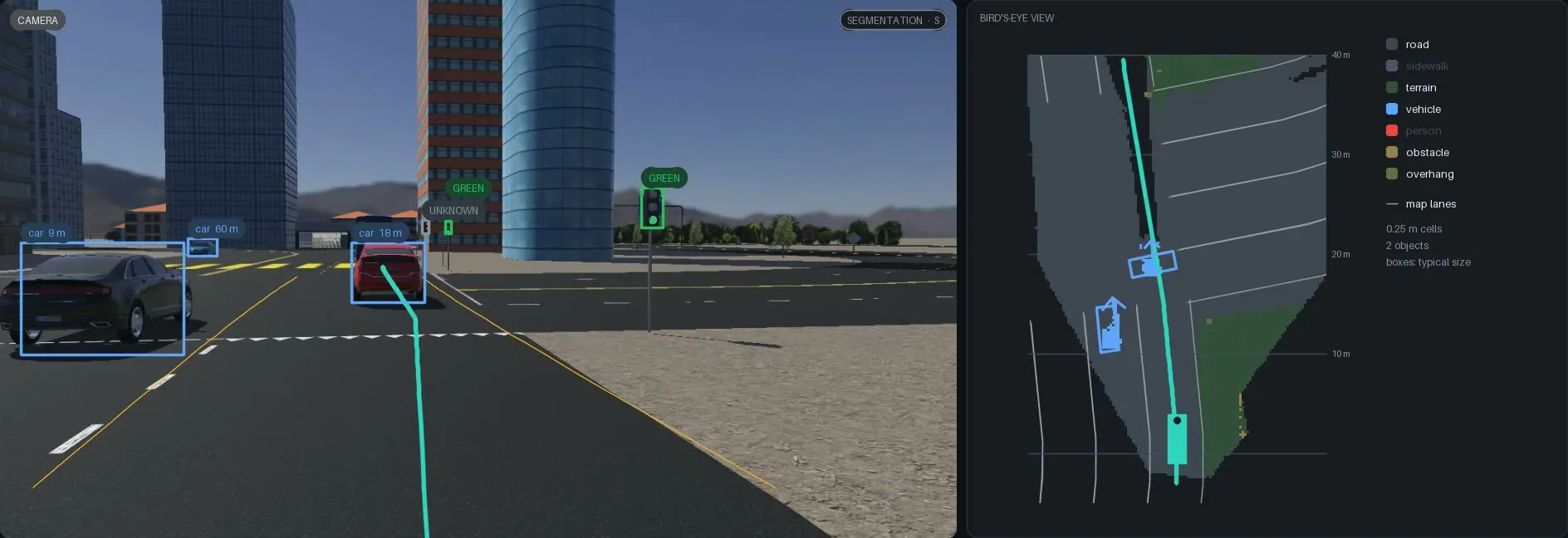
One frame of a drive. Left: the camera with tracked vehicles, a STOP sign, light states and the planned path. Right: the 0.25 m grid built from that frame. The car that turns across our path is in the grid with its velocity.
Each depth pixel is projected into the ground plane with its segmentation class and voted into a 0.25 m grid in the car’s frame. Static classes are kept for 2 s and moved with the car’s motion, so the grid also holds road that the camera saw a moment ago. A cost map prices each cell for the planner.
The pretrained segmentation model called the sandy roadside “road”, so the grid had no road edge. I fine-tuned it on labels from the simulator. The simulator does not label the ground, so the map decided which ground pixels are road and which are terrain. On roads never used for training, the terrain IoU went from 0 to 0.86, and the road IoU in the grid went from 0.79 to 0.97.
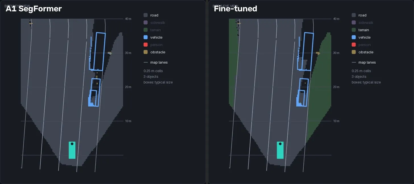
The same frame in the grid. Left: the pretrained model labels the terrain as road. Right: after fine-tuning, the road edge is back.
The dashboard, at twice real speed: the car approaches a red light, waits at the line and moves off on green. A recorded drive replayed through the agent. Everything drawn comes from what the car perceived; no ground truth is shown.
Planning and behaviour
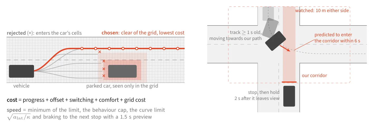
Left: candidate paths that enter occupied cells are rejected, and the cheapest clear path is kept. Right: the car stops for a tracked vehicle that is predicted to enter its path within 6 s.
The planner samples paths that blend to a lateral offset, gives each a speed profile, and keeps the cheapest path that stays clear of the grid. A behaviour state machine sits above it. Each active rule (a STOP line, a red light, a lead car, a crossing car, a pedestrian) gives a speed limit and a stop distance, and the most restrictive one controls the car. The crossing-car rule came last. In the final test drives, a car that turned across our path on a green light hit us on two of three seeds. With the rule, all three seeds stop for that car and complete the loop.
At four times real speed, then in real time: the car waits behind the lead car at a red light, moves off on green, and brakes for a car that crosses on our green.
Localisation and distance
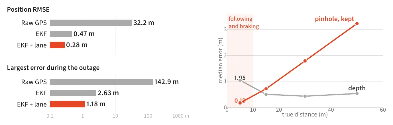
Left: position error in a simulated drive with a 20 s GPS outage, on a log scale. Right: median distance error for 10,260 tracked vehicles. Below 10 m the pinhole estimate from the image is better than the range finder, so the car uses it there.
An extended Kalman filter predicts the pose from wheel speed and the gyro. GPS corrects it, and the lane offset against the map holds it on the road. In the Webots city its position error is 0.08 to 0.10 m, against about 0.7 m for raw GPS.
Results
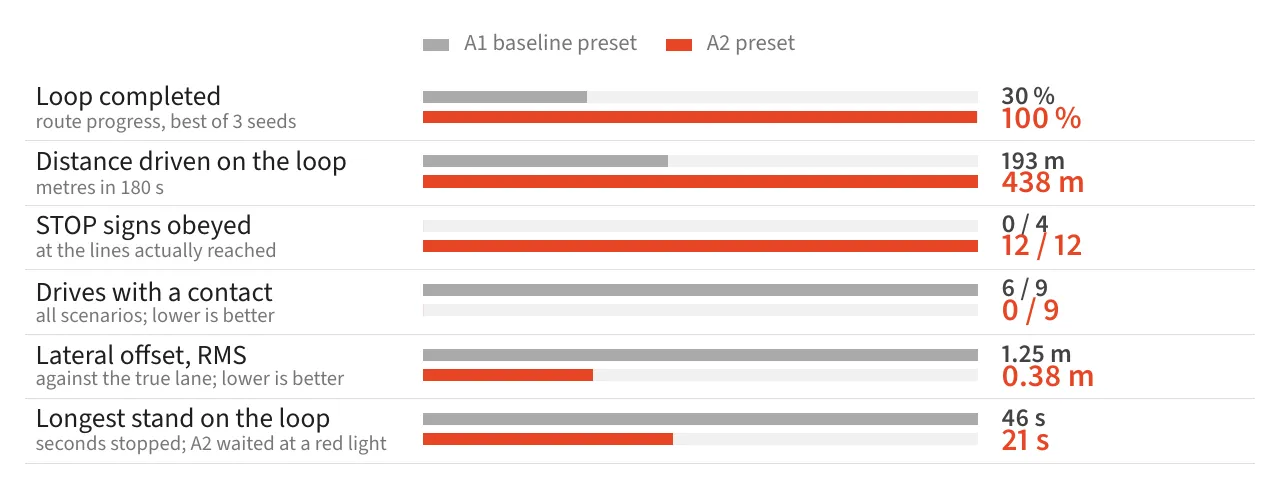
The baseline preset against the extended system: three scenarios, seeds 1, 2 and 7, 18 drives in total. Each drive is scored frame by frame against the simulator's ground truth and the map. Each row has its own scale.
On the city loop the extended system completed the route on every seed and stopped at all 12 STOP signs. No drive came into contact with another road user; the baseline did in 6 of 9 drives. The lateral error from the lane centre fell from 1.25 m to 0.38 m RMS.
What this is not
This is one simulated world. The models were fine-tuned on it, and we have not measured how they transfer to another. Neither system completes the second route, which turns through a junction lane of about 2.3 m radius, tighter than the car can steer. The car has one forward camera, so it sees side traffic only when it enters the image, and the background traffic does not react to the car. One step takes about 130 ms on a laptop GPU, so the simulation runs at about 0.8 times real time. This was the group project of ELEC5308 at the University of Sydney, Group 5.